Introduction to Bayesian Optimisation

In this guide we introduce the Bayesian Optimisation (BO) paradigm for optimising black-box functions. We'll assume an understanding of Gaussian processes (GPs), so if you're not familiar with them, the GP introduction notebook in GPJax is a great place to start.

%load_ext jaxtyping
%jaxtyping.typechecker beartype.beartype

from typing import (
    List,
    Tuple,
)

import jax
from jax import config

# Enable float64 for stable matrix operations
config.update("jax_enable_x64", True)
import equinox as eqx
import gpjax as gpx
import jax.numpy as jnp
import jax.random as jr
import matplotlib as mpl
import matplotlib.pyplot as plt
import paramax
from decijax.acquisition_functions import ExpectedImprovement
from decijax.acquisition_functions.base import SinglePointAcquisitionFunction
from decijax.acquisition_maximizer import ContinuousSinglePointAcquisitionMaximizer
from decijax.models.builder import GPJaxConjugateGPBuilder
from decijax.models.gps import GPJaxConjugateGP
from decijax.search_space import ContinuousSearchSpace
from decijax.utils import OBJECTIVE
from jaxtyping import Array, Float
from matplotlib import cm

key = jr.key(44)
cols = mpl.rcParams["axes.prop_cycle"].by_key()["color"]

/home/runner/work/decijax/decijax/.venv/lib/python3.13/site-packages/tqdm/auto.py:21: TqdmWarning: IProgress not found. Please update jupyter and ipywidgets. See https://ipywidgets.readthedocs.io/en/stable/user_install.html
  from .autonotebook import tqdm as notebook_tqdm

Motivating Examples

Countless problems in the physical world involve optimising functions for which the explicit functional form is unknown, but which can be expensively queried throughout their domain. Many exciting problems in the natural sciences have these characteristics, such as the task of designing new molecules with optimised properties (Griffiths and Lobato, 2020). Here, the domain being optimised over is the space of possible molecules, with the objective function depending on the property being optimised, for instance within drug-design this may be the efficacy of the drug. The function from molecules to efficacy is unknown, but can be queried by synthesising a molecule and running an experiment to measure its efficacy. This is clearly an expensive procedure!

Within the domain of machine learning, the task of optimising neural network architectures is another example of such a problem (commonly referred to as Neural Architecture Search (NAS)). Here, the domain is the space of possible neural network architectures, and the objective function is a metric such as the accuracy of the trained model. Again, the function from neural network architectures to accuracy is unknown, but can be queried by training a model with a given architecture and evaluating its accuracy. This is also an expensive procedure, as training models can be incredibly time consuming and computationally demanding.

Finally, these problems are ubiquitous within the field of climate science, with (Hellan et al., 2023) providing several excellent examples. One such example is the task of deciding where to place wind turbines in a wind farm in order to maximise the energy generated. Here, the domain is the space of possible locations for the wind turbines, and the objective function is the energy generated by the wind farm. The function from locations to energy generated is unknown, but could be queried by running a simulation of the wind farm with the turbines placed at a given set of locations. Running such simulations can be expensive, particularly if they are high-fidelity.

At the heart of all these problems is the task of optimising a function for which we don't have the explicit functional form, but which we can (expensively) query at any point in its domain. Bayesian optimisation provides a principled framework for solving such problems.

What is Bayesian Optimisation?

Bayesian optimisation (BO) (Močkus, 1974) provides a principled method for making decisions under uncertainty. The aim of BO is to find the global maximum of a black-box objective function, \(\max_{\mathbf{x} \in \mathcal{X}} f(\mathbf{x})\). The function \(f\) is said to be a black-box function because its explicit functional form is unknown. However, it is assumed that one is able to ascertain information about the function by evaluating it at points in its domain, \(X\). However, these evaluations are assumed to be expensive, as seen in the motivating examples. Therefore, the goal of BO is to maximise \(f\) with as few evaluations of the black-box function as possible.

As such, BO can be thought of as sequential decision-making problem. At each iteration one must choose which point (or batch of points) in a function's domain to evaluate next, drawing on previously observed values to make optimal decisions. In order to do this effectively, we need a way of representing our uncertainty about the black-box function \(f\), which we can update in light of observing more data. Gaussian processes will be an ideal tool for this purpose!

Surrogate models lie at the heart of BO, and are used to model the black-box function. GPs are a natural (though by no means the only) choice for this model, as they not only provide point estimates for the values taken by the function throughout its domain, but crucially provide a full predictive posterior distribution of the range of values the function may take. This rich quantification of uncertainty enables BO to balance exploration and exploitation in order to efficiently converge upon minima.

Having chosen a surrogate model which we can use to express our current beliefs about the black-box function, ideally we would like a method which can use the surrogate model's posterior distribution to automatically decide which point(s) in the black-box function's domain to query next. This is where acquisition functions come in. The acquisition function \(\alpha: \mathcal{X} \to \mathbb{R}\) is defined over the same domain as the surrogate model, and typically uses the surrogate model's posterior distribution to quantify the expected utility of evaluating the black-box function at a given point, with the expectation taking place with respect to the model's posterior. Simply put, for each point in the black-box function's domain, \(\mathbf{x} \in \mathcal{X}\), the acquisition function quantifies how useful it would be to evaluate the black-box function at \(\mathbf{x}\) in order to find the maximum of the black-box function, given the datapoints observed so far. Therefore, in order to decide which point to query next we simply choose the point which maximises the acquisition function, using an optimiser which depends on the domain. In this notebook we'll be operating on the Euclidean domain, \(\mathbb{R}^D\), and so a suitable optimiser is L-BFGS (Liu and Nocedal, 1989).

The Bayesian optimisation loop can be summarised as follows, with \(i\) denoting the current iteration:

Select the next point to query, \(\mathbf{x}_{i}\), by maximising the acquisition function \(\alpha\), defined using the surrogate model \(\mathcal{M}_i\) conditioned on previously observed data \(\mathcal{D}_i\):

\[\mathbf{x}_{i} = \arg\max_{\mathbf{x} \in \mathcal{X}} \alpha (\mathbf{x}; \mathcal{D}_i, \mathcal{M}_i)\]

Evaluate the objective function at \(\mathbf{x}_i\), yielding observation \(y_i = f(\mathbf{x}_i)\).
Append the most recent observation to the dataset, \(\mathcal{D}_{i+1} = \mathcal{D}_i \cup \{(\mathbf{x}_i, y_i)\}\).
Condition the model on the updated dataset to yield \(\mathcal{M}_{i+1}\).

This process is repeated until some stopping criterion is met, such as a function evaluation budget being exhausted.

There are a plethora of acquisition functions to choose from, each with their own advantages and disadvantages, of which (Shahriari et al., 2015) provides an excellent overview.

In this guide we will focus on Expected Improvement (EI), a conceptually simple yet effective method for characterising the utility of querying points in a black-box function's domain, which will be useful in demonstrating the key aspects of BO.

Expected Improvement

Expected Improvement (Močkus, 1974) is a simple method which naturally balances exploration and exploitation. With this method, the utility of observing a point \(f\), given current best observation \(f^*\), is simply defined as the amount by which \(f\) improves over \(f^*\) if it is better, and \(0\) otherwise. Mathematically, the utility \(u(f;f^*) = \text{ReLU}(f - f^*)\). Expected improvement is then defined as the expectation of this utility with respect to the model's posterior over \(f\) throughout the domain. For Gaussian predictives, this integral is analytically tractable, yielding the following acquisition function:

\[ \begin{aligned} \alpha_{\text{EI}}(\mathbf{x};\mathcal{D}_i, \mathcal{M}_i, f^*) &= \mathbb{E}_{f}[\text{ReLU}(f - f^*)] \\ &= \underbrace{(\mu_{\mathcal{M}_i}(\mathbf{x}) - f^*)\Phi \left(\frac{\mu_{\mathcal{M}_i}(\mathbf{x}) - f^*}{\sigma_{\mathcal{M}_i}(\mathbf{x})}\right)}_\text{exploits areas with high mean} \\ &+ \underbrace{\sigma_{\mathcal{M}_i}(\mathbf{x}) \phi \left(\frac{\mu_{\mathcal{M}_i}(\mathbf{x}) - f^*}{\sigma_{\mathcal{M}_i}(\mathbf{x})}\right)}_\text{explores areas with high variance} \nonumber \end{aligned} \]

with \(\Phi(\cdot)\) denoting the standard normal cumulative distribution function and \(\phi(\cdot)\) being the standard normal probability density function.

Objective Function

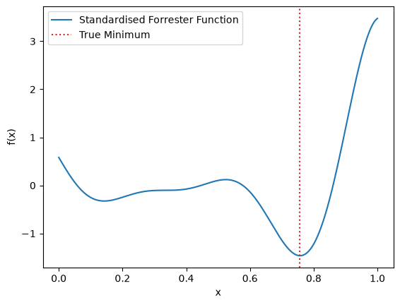
As a toy example, we shall be applying BO to the widely used Forrester function over the domain \(\mathbf{x} \in [0, 1]\):

\[f(x) = (6x - 2)^2 \sin(12x - 4)\]

treating \(f\) as a black-box function. Note that we'll be minimising this function, but the BO component of decijax has been written to maximise the function, so we'll maximise the negative of the Forrester function. The global minimum of this (standardised) function is located at \(x = 0.757\), where \(f(x) = -1.463\).

We also note a few other common tricks: - We standardise the output of the function, such that it has a mean of 0 and standard deviation of 1. This is quite common practice when using GPs; we're using a zero mean prior, so ensuring that our data has a mean of zero aligns with this, and often we have scale parameters in the covariance function, which are frequently initialised, or have priors set on them, under the assumption that the function being modelled has unit variance. - Covariance functions often have hyperpriors which have been set based on the assumption that the domain of the problem of interest is the unit hypercube (see Hvarfner et al. 2024 for a good example).

def neg_standardised_forrester(x: Float[Array, "N 1"]) -> Float[Array, "N 1"]:
    mean = 0.45321
    std = 4.4258
    return -((6 * x - 2) ** 2 * jnp.sin(12 * x - 4) - mean) / std

plt_x = jnp.linspace(0, 1, 500).reshape(-1, 1)
plt_y = -neg_standardised_forrester(plt_x)

fig, ax = plt.subplots()
ax.plot(plt_x, plt_y, color=cols[0], label="Standardised Forrester Function")
ax.axvline(x=0.757, linestyle=":", color=cols[3], label="True Minimum")
ax.set_xlabel("x")
ax.set_ylabel("f(x)")
ax.legend()
plt.show()

png

We'll first go through one iteration of the BO loop step-by-step, before wrapping this up in a loop to perform the full optimisation. We'll be combining components from the decijax library in order to do this. Note that decijax provides functionality for running the entire BO loop end-to-end without stitching the components together manually (via its DecisionMaker). In this notebook we expose the individual components for educational purposes.

First we'll specify the domain over which we wish to optimise the function, as well as sampling some initial points for fitting our surrogate model using a space-filling design. We do this using the SearchSpace abstraction from decijax:

lower_bound = jnp.array([0.0])
upper_bound = jnp.array([1.0])
search_space = ContinuousSearchSpace(lower_bounds=lower_bound, upper_bounds=upper_bound)

initial_sample_num = 5
key, subkey = jr.split(key)
initial_x = search_space.sample(initial_sample_num, key=subkey)
initial_y = neg_standardised_forrester(initial_x)
dataset = gpx.Dataset(X=initial_x, y=initial_y)

/home/runner/work/decijax/decijax/src/decijax/search_space.py:84: UserWarning: The balance properties of Sobol' points require n to be a power of 2.
  initial_sample = jnp.array(sampler.random(num_points))

Next we'll define our GP model, using a Matérn52 kernel and zero mean function, and fit the kernel parameters by minimising the negative log-marginal likelihood. We'll use the GPJaxConjugateGPBuilder for this, which builds and trains a GP when the build() method is called with a dataset.

mean = gpx.mean_functions.Zero()
kernel = gpx.kernels.Matern52()
prior = gpx.gps.Prior(mean_function=mean, kernel=kernel)


def likelihood_builder(n: int) -> gpx.likelihoods.Gaussian:
    # Our function is noise-free, so we fix the observation noise's standard
    # deviation at a very small value rather than treating it as trainable.
    likelihood = gpx.likelihoods.Gaussian(num_datapoints=n, obs_stddev=1e-6)
    return eqx.tree_at(
        lambda l: l.obs_stddev,  # noqa: E741
        likelihood,
        replace_fn=paramax.non_trainable,
    )


gp_builder = GPJaxConjugateGPBuilder(
    prior=prior,
    likelihood_builder=likelihood_builder,
    optimization_objective=gpx.objectives.conjugate_mll,
    observation_transform=lambda x: x,
)
key, subkey = jr.split(key)
opt_posterior = gp_builder.build(dataset, subkey)

Next we'll set up our acquisition function, using the pre-implemented ExpectedImprovement acquisition function from the acquisition_functions subpackage of decijax. The primary method of acquisition functions is build_acquisition_function, which takes a dictionary of models (keyed by their role - in this case just OBJECTIVE), and returns a function mapping any batch of query points [N, D] to their acquisition values [N, 1]. Because it returns a pure function, this can be easily composed with JAX transforms such as jax.grad or jax.jit, facilitating the use of gradient-based optimisers such as L-BFGS.

ei = ExpectedImprovement()

In order to maximise the acquisition function, we'll be using the L-BFGS-B (Byrd et al., 1995) optimiser from scipy (currently there is no JAX-native L-BFGS-B implementation). This is a gradient-based optimiser which performs optimisation within a bounded domain. In order to perform optimisation, this optimiser requires a point to start from. Therefore, we will first query the acquisition function at a random set of points, and then use the highest point from this set of points as the starting point for the optimiser. In this example we'll sample 100 points from the acquisition function, due to the simple nature of the Forrester function. However, in practice it can be beneficial to adopt a more sophisticated approach, and there are several heuristics available in the literature (see for example (Le Riche and Picheny, 2021)). For instance, one may randomly sample the acquisition function at a number of points proportional to the dimensionality of the input space, and one may run gradient-based optimisation from multiple of these points, to reduce the impact of converging upon local minima.

We'll use the ContinuousSinglePointAcquisitionMaximizer from decijax in order to do this, which implements the functionality above. We specify num_initial_samples=100, to sample the acquisition function randomly at 100 points, and num_optimization_runs=1, signifying that the gradient-based optimiser will be run from the best of these points.

acq_maximizer = ContinuousSinglePointAcquisitionMaximizer(
    num_initial_samples=100, num_optimization_runs=1
)

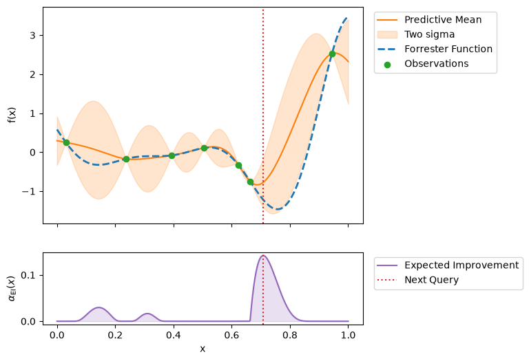
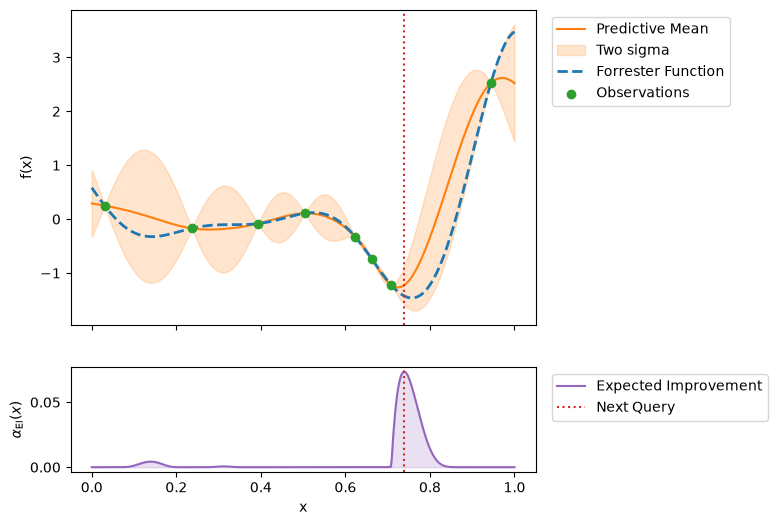
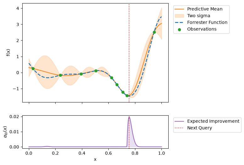
To visualise a single step of the loop, we define a plot_bo_step helper. It shows the surrogate's predictive posterior on top and the acquisition function directly below, sharing an x axis so that the acquisition function's peak lines up with the posterior, and marks the next point to query in both panels. We'll reuse it on every iteration of the BO loop further down.

def plot_bo_step(
    posterior: GPJaxConjugateGP,
    dataset: gpx.Dataset,
    next_query: Float[Array, "1 1"],
    acquisition_fn: SinglePointAcquisitionFunction,
) -> None:
    """Plot a single step of the BO loop.

    The top panel shows the surrogate's predictive posterior and the bottom panel the
    acquisition function, sharing an x axis, with the next point to query marked in
    both. The posterior is displayed in the original *minimisation* space (via
    negation).
    """
    plt_x = jnp.linspace(0, 1, 500).reshape(-1, 1)

    latent_dist = posterior.predict(plt_x)
    predictive_mean = latent_dist.mean[0]
    predictive_std = latent_dist.stddev[0]
    acquisition_values = acquisition_fn(plt_x)  # [N, 1]
    next_x = float(next_query[0, 0])

    fig, (ax, ax_acq) = plt.subplots(
        2,
        1,
        sharex=True,
        figsize=(6, 6),
        gridspec_kw={"height_ratios": [3, 1]},
    )

    # Top panel: posterior predictive in the original (minimisation) space.
    ax.plot(plt_x, -predictive_mean, label="Predictive Mean", color=cols[1])
    ax.fill_between(
        plt_x.squeeze(),
        -predictive_mean - 2 * predictive_std,
        -predictive_mean + 2 * predictive_std,
        alpha=0.2,
        label="Two sigma",
        color=cols[1],
    )
    ax.plot(
        plt_x,
        -neg_standardised_forrester(plt_x),
        label="Forrester Function",
        color=cols[0],
        linestyle="--",
        linewidth=2,
    )
    ax.scatter(dataset.X, -dataset.y, label="Observations", color=cols[2], zorder=2)
    ax.axvline(x=next_x, linestyle=":", color=cols[3])
    ax.set_ylabel("f(x)")
    ax.legend(loc="upper left", bbox_to_anchor=(1.02, 1.0))

    # Bottom panel: acquisition function, sharing the x axis with the panel above.
    ax_acq.plot(plt_x, acquisition_values, color=cols[4], label="Expected Improvement")
    ax_acq.fill_between(
        plt_x.squeeze(),
        0.0,
        acquisition_values.squeeze(),
        alpha=0.2,
        color=cols[4],
    )
    ax_acq.axvline(x=next_x, linestyle=":", color=cols[3], label="Next Query")
    ax_acq.set_xlabel("x")
    ax_acq.set_ylabel(r"$\alpha_{\mathrm{EI}}(x)$")
    ax_acq.legend(loc="upper left", bbox_to_anchor=(1.02, 1.0))

    plt.show()

acquisition_function = ei.build_acquisition_function({OBJECTIVE: opt_posterior}, key)
key, subkey = jr.split(key)
next_query = acq_maximizer.maximize(acquisition_function, search_space, subkey)
plot_bo_step(opt_posterior, dataset, next_query, acquisition_function)

/home/runner/work/decijax/decijax/src/decijax/search_space.py:84: UserWarning: The balance properties of Sobol' points require n to be a power of 2.
  initial_sample = jnp.array(sampler.random(num_points))

png

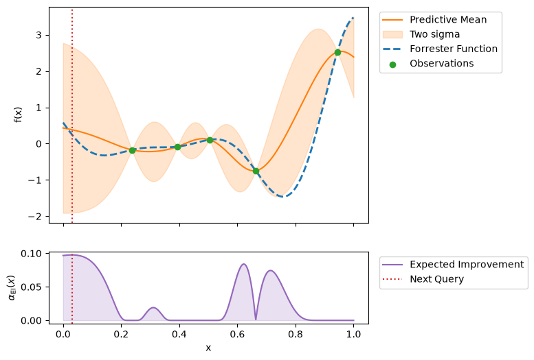
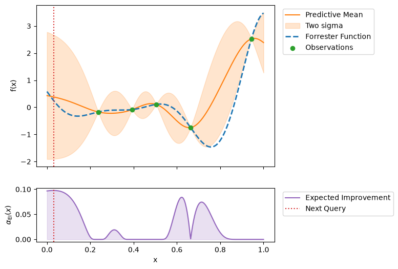
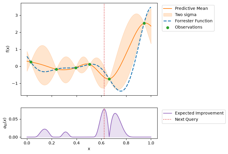
Having found the minimum of the sample from the posterior, we can then evaluate the black-box objective function at this point, append the new observation to our dataset, and update our model with the newly augmented dataset, repeating the whole process until some stopping criterion is met. Below we repeat this process for 5 iterations, plotting the progress at each iteration.

bo_iters = 5
for _ in range(bo_iters):
    key, subkey = jr.split(key)
    opt_posterior = gp_builder.build(dataset, subkey)

    key, subkey = jr.split(key)
    acquisition_function = ei.build_acquisition_function(
        {OBJECTIVE: opt_posterior}, subkey
    )

    key, subkey = jr.split(key)
    query_x = acq_maximizer.maximize(acquisition_function, search_space, subkey)
    plot_bo_step(opt_posterior, dataset, query_x, acquisition_function)

    # Evaluate the black-box function at the queried point, and add it to the dataset.
    query_y = neg_standardised_forrester(query_x)
    dataset = dataset + gpx.Dataset(X=query_x, y=query_y)

png

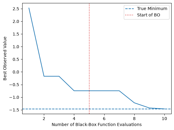
Below we plot the best observed black-box function value against the number of times the black-box function has been evaluated. Note that the first 5 samples are randomly sampled to fit the initial GP model, and we denote the start of using BO to sample with the dotted vertical line.

We can see that the BO algorithm quickly converges to the global minimum of the black-box function!

fig, ax = plt.subplots()
fn_evaluations = jnp.arange(1, bo_iters + initial_sample_num + 1)
cumulative_best_y = -jax.lax.associative_scan(jax.numpy.maximum, dataset.y)
ax.plot(fn_evaluations, cumulative_best_y)
ax.axhline(y=-1.463, linestyle="--", label="True Minimum")
ax.axvline(x=initial_sample_num, linestyle=":", color=cols[3], label="Start of BO")
ax.set_xlabel("Number of Black-Box Function Evaluations")
ax.set_ylabel("Best Observed Value")
ax.legend()
plt.show()

png

A More Challenging Example - The Six-Hump Camel Function

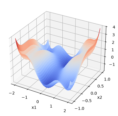
We'll now apply BO to a more challenging example, the Six-Hump Camel Function. This is a function of two inputs defined as follows:

\[f(x_1, x_2) = (4 - 2.1x_1^2 + \frac{x_1^4}{3})x_1^2 + x_1x_2 + (-4 + 4x_2^2)x_2^2\]

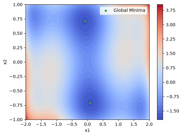
We'll be evaluating it over the domain \(x_1 \in [-2, 2]\) and \(x_2 \in [-1, 1]\), and shall standardise it. The global minima of this function are located at \(\mathbf{x} = (0.0898, -0.7126)\) and \(\mathbf{x} = (-0.0898, 0.7126)\), where the standardised function takes the value \(f(\mathbf{x}) = -1.8377\). Note that we once again try to maximise the negative of this function, due to the maximisation convention of decijax, though plots show the original function.

def neg_standardised_six_hump_camel(x: Float[Array, "N 2"]) -> Float[Array, "N 1"]:
    mean = 1.12767
    std = 1.17500
    x1 = x[..., :1]
    x2 = x[..., 1:]
    term1 = (4 - 2.1 * x1**2 + x1**4 / 3) * x1**2
    term2 = x1 * x2
    term3 = (-4 + 4 * x2**2) * x2**2
    return -(term1 + term2 + term3 - mean) / std

First, we'll visualise the function over the domain of interest:

x1 = jnp.linspace(-2, 2, 100)
x2 = jnp.linspace(-1, 1, 100)
x1, x2 = jnp.meshgrid(x1, x2)
x = jnp.stack([x1.flatten(), x2.flatten()], axis=1)
y = -neg_standardised_six_hump_camel(x)

fig, ax = plt.subplots(subplot_kw={"projection": "3d"})
surf = ax.plot_surface(
    x1,
    x2,
    y.reshape(x1.shape[0], x2.shape[0]),
    linewidth=0,
    cmap=cm.coolwarm,
    antialiased=False,
)
ax.set_xlabel("x1")
ax.set_ylabel("x2")
plt.show()

png

For more clarity, we can generate a contour plot of the function which enables us to see the global minima of the function more clearly.

x_star_one = jnp.array([[0.0898, -0.7126]])
x_star_two = jnp.array([[-0.0898, 0.7126]])
fig, ax = plt.subplots()
contour_plot = ax.contourf(
    x1, x2, y.reshape(x1.shape[0], x2.shape[0]), cmap=cm.coolwarm, levels=40
)
ax.scatter(
    x_star_one[0][0], x_star_one[0][1], marker="*", color=cols[2], label="Global Minima"
)
ax.scatter(x_star_two[0][0], x_star_two[0][1], marker="*", color=cols[2])
ax.set_xlabel("x1")
ax.set_ylabel("x2")
fig.colorbar(contour_plot)
ax.legend()
plt.show()

png

Next, we'll run the BO loop using Expected Improvement as before. This time we'll run the experiment 5 times in order to see how the algorithm performs on average, with different starting points for the initial GP model. This is good practice, as the performance obtained is likely to vary between runs depending on the initialisation samples used to fit the initial GP model.

lower_bound = jnp.array([-2.0, -1.0])
upper_bound = jnp.array([2.0, 1.0])
camel_search_space = ContinuousSearchSpace(
    lower_bounds=lower_bound, upper_bounds=upper_bound
)

camel_prior = gpx.gps.Prior(
    mean_function=gpx.mean_functions.Zero(),
    kernel=gpx.kernels.Matern52(active_dims=[0, 1]),
)
camel_gp_builder = GPJaxConjugateGPBuilder(
    prior=camel_prior,
    likelihood_builder=likelihood_builder,
    optimization_objective=gpx.objectives.conjugate_mll,
    observation_transform=lambda x: x,
)

camel_acq_maximizer = ContinuousSinglePointAcquisitionMaximizer(
    num_initial_samples=1000, num_optimization_runs=1
)

initial_sample_num = 5
bo_iters = 12
num_experiments = 5
bo_experiment_results = []

for experiment in range(num_experiments):
    print(f"Starting Experiment: {experiment + 1}")

    # Set up the initial dataset using a space-filling design.
    key, subkey = jr.split(key)
    initial_x = camel_search_space.sample(initial_sample_num, key=subkey)
    initial_y = neg_standardised_six_hump_camel(initial_x)
    dataset = gpx.Dataset(X=initial_x, y=initial_y)

    for i in range(bo_iters):
        # Refit the surrogate to all data observed so far.
        key, subkey = jr.split(key)
        opt_posterior = camel_gp_builder.build(dataset, subkey)

        # Build the EI acquisition function and maximise it to pick the next point.
        key, subkey = jr.split(key)
        acquisition_function = ei.build_acquisition_function(
            {OBJECTIVE: opt_posterior}, subkey
        )
        key, subkey = jr.split(key)
        query_x = camel_acq_maximizer.maximize(
            acquisition_function, camel_search_space, subkey
        )

        # Evaluate the black-box function at the queried point and add it to the dataset.
        query_y = neg_standardised_six_hump_camel(query_x)
        print(
            f"BO Iteration: {i + 1}, Queried Point: {query_x}, "
            f"Black-Box Function Value: {query_y}"
        )
        dataset = dataset + gpx.Dataset(X=query_x, y=query_y)

    bo_experiment_results.append(dataset)

Starting Experiment: 1


/home/runner/work/decijax/decijax/src/decijax/search_space.py:84: UserWarning: The balance properties of Sobol' points require n to be a power of 2.
  initial_sample = jnp.array(sampler.random(num_points))


BO Iteration: 1, Queried Point: [[ 0.52093722 -0.10897378]], Black-Box Function Value: [[0.25009812]]


BO Iteration: 2, Queried Point: [[ 0.31447418 -0.2071478 ]], Black-Box Function Value: [[0.83551315]]


BO Iteration: 3, Queried Point: [[ 0.11056357 -0.44968469]], Black-Box Function Value: [[1.50987595]]


BO Iteration: 4, Queried Point: [[ 0.23368512 -0.79056813]], Black-Box Function Value: [[1.73420362]]


BO Iteration: 5, Queried Point: [[ 0.60034721 -1.        ]], Black-Box Function Value: [[0.46258261]]


BO Iteration: 6, Queried Point: [[ 0.11308833 -0.73781242]], Black-Box Function Value: [[1.83184773]]


BO Iteration: 7, Queried Point: [[ 0.07991425 -0.89542237]], Black-Box Function Value: [[1.5399828]]


BO Iteration: 8, Queried Point: [[ 0.15986386 -0.68113191]], Black-Box Function Value: [[1.81318934]]


BO Iteration: 9, Queried Point: [[ 0.08257372 -0.69436154]], Black-Box Function Value: [[1.83536481]]


BO Iteration: 10, Queried Point: [[-0.58659945  1.        ]], Black-Box Function Value: [[0.48760971]]


BO Iteration: 11, Queried Point: [[-1.56173027  1.        ]], Black-Box Function Value: [[0.50162095]]


BO Iteration: 12, Queried Point: [[-0.29694041  0.24113474]], Black-Box Function Value: [[0.92062672]]
Starting Experiment: 2


BO Iteration: 1, Queried Point: [[-0.31103987  1.        ]], Black-Box Function Value: [[0.91155771]]


BO Iteration: 2, Queried Point: [[-0.09542556  0.56044133]], Black-Box Function Value: [[1.70779294]]


BO Iteration: 3, Queried Point: [[0.08916321 0.7714415 ]], Black-Box Function Value: [[1.6944896]]


BO Iteration: 4, Queried Point: [[ 0.34272554 -1.        ]], Black-Box Function Value: [[0.87573272]]


BO Iteration: 5, Queried Point: [[ 0.00589937 -0.56601016]], Black-Box Function Value: [[1.70365834]]


BO Iteration: 6, Queried Point: [[-0.12373467 -0.82112702]], Black-Box Function Value: [[1.56924804]]


BO Iteration: 7, Queried Point: [[ 0.069946   -0.70275334]], Black-Box Function Value: [[1.83587621]]


BO Iteration: 8, Queried Point: [[ 0.25419692 -0.52503346]], Black-Box Function Value: [[1.5404529]]


BO Iteration: 9, Queried Point: [[-0.06341291  0.71933748]], Black-Box Function Value: [[1.83490802]]


BO Iteration: 10, Queried Point: [[-0.18048406  0.67772474]], Black-Box Function Value: [[1.80024245]]


BO Iteration: 11, Queried Point: [[ 2. -1.]], Black-Box Function Value: [[-0.51545816]]


BO Iteration: 12, Queried Point: [[-0.39854188  0.27580029]], Black-Box Function Value: [[0.79575257]]
Starting Experiment: 3


BO Iteration: 1, Queried Point: [[ 0.25244662 -1.        ]], Black-Box Function Value: [[0.96480183]]


BO Iteration: 2, Queried Point: [[-0.31025746 -1.        ]], Black-Box Function Value: [[0.38428504]]


BO Iteration: 3, Queried Point: [[ 0.06326459 -0.82742751]], Black-Box Function Value: [[1.72568392]]


BO Iteration: 4, Queried Point: [[ 0.07941127 -0.66911906]], Black-Box Function Value: [[1.82530363]]


BO Iteration: 5, Queried Point: [[-0.0076759  -0.69451988]], Black-Box Function Value: [[1.80498577]]


BO Iteration: 6, Queried Point: [[ 0.06218404 -0.7188115 ]], Black-Box Function Value: [[1.83473902]]


BO Iteration: 7, Queried Point: [[-0.08007891 -0.29823575]], Black-Box Function Value: [[1.19349536]]


BO Iteration: 8, Queried Point: [[ 0.1266598  -0.71936146]], Black-Box Function Value: [[1.83313202]]


BO Iteration: 9, Queried Point: [[ 2. -1.]], Black-Box Function Value: [[-0.51545816]]


BO Iteration: 10, Queried Point: [[ 0.27205114 -0.624908  ]], Black-Box Function Value: [[1.67237919]]


BO Iteration: 11, Queried Point: [[-0.12186476  1.        ]], Black-Box Function Value: [[1.01327043]]


BO Iteration: 12, Queried Point: [[-0.67259348  1.        ]], Black-Box Function Value: [[0.33160807]]
Starting Experiment: 4


BO Iteration: 1, Queried Point: [[ 0.43698239 -0.77771005]], Black-Box Function Value: [[1.47573903]]


BO Iteration: 2, Queried Point: [[ 0.02393492 -0.84753562]], Black-Box Function Value: [[1.66384364]]


BO Iteration: 3, Queried Point: [[ 0.04917422 -0.55536549]], Black-Box Function Value: [[1.70087194]]


BO Iteration: 4, Queried Point: [[ 0.14622223 -0.67167789]], Black-Box Function Value: [[1.81427438]]


BO Iteration: 5, Queried Point: [[ 0.12950682 -0.71459293]], Black-Box Function Value: [[1.83256396]]


BO Iteration: 6, Queried Point: [[ 0.17315034 -0.77934212]], Black-Box Function Value: [[1.78591574]]


BO Iteration: 7, Queried Point: [[ 0.08841065 -0.7064311 ]], Black-Box Function Value: [[1.83743384]]


/home/runner/work/decijax/decijax/src/decijax/search_space.py:84: UserWarning: The balance properties of Sobol' points require n to be a power of 2.
  initial_sample = jnp.array(sampler.random(num_points))


BO Iteration: 8, Queried Point: [[-0.36408832 -0.63227199]], Black-Box Function Value: [[1.16014064]]


BO Iteration: 9, Queried Point: [[ 2. -1.]], Black-Box Function Value: [[-0.51545816]]


BO Iteration: 10, Queried Point: [[-2.  1.]], Black-Box Function Value: [[-0.51545816]]


BO Iteration: 11, Queried Point: [[ 0.71253855 -0.2743129 ]], Black-Box Function Value: [[0.05814404]]


BO Iteration: 12, Queried Point: [[ 0.09290881 -0.70655059]], Black-Box Function Value: [[1.83739606]]
Starting Experiment: 5


BO Iteration: 1, Queried Point: [[-0.37569002  0.54666164]], Black-Box Function Value: [[1.40213434]]


BO Iteration: 2, Queried Point: [[-0.25280155  0.70821319]], Black-Box Function Value: [[1.75281118]]


BO Iteration: 3, Queried Point: [[0.19251474 1.        ]], Black-Box Function Value: [[0.67214904]]


BO Iteration: 4, Queried Point: [[-0.30306564  0.83677004]], Black-Box Function Value: [[1.59236951]]


BO Iteration: 5, Queried Point: [[-0.15371599  0.68390739]], Black-Box Function Value: [[1.8172643]]


BO Iteration: 6, Queried Point: [[-0.07624424  0.59308706]], Black-Box Function Value: [[1.75472176]]


BO Iteration: 7, Queried Point: [[-0.11099126  0.70135258]], Black-Box Function Value: [[1.83514307]]


BO Iteration: 8, Queried Point: [[-0.06290651  0.68844521]], Black-Box Function Value: [[1.83188821]]


BO Iteration: 9, Queried Point: [[2.         0.54056611]], Black-Box Function Value: [[-2.43361654]]


BO Iteration: 10, Queried Point: [[ 1.07114411 -1.        ]], Black-Box Function Value: [[-0.11028279]]


BO Iteration: 11, Queried Point: [[-2.         -0.06281292]], Black-Box Function Value: [[-2.31112306]]


BO Iteration: 12, Queried Point: [[ 2. -1.]], Black-Box Function Value: [[-0.51545816]]

We'll also run a random benchmark, whereby we randomly sample from the search space for 17 iterations. This is a useful benchmark to compare the performance of BO against in order to ascertain how much of an advantage BO provides over such a simple approach.

random_experiment_results = []
for i in range(num_experiments):
    key, subkey = jr.split(key)
    initial_x = bo_experiment_results[i].X[:5]
    initial_y = bo_experiment_results[i].y[:5]
    final_x = jr.uniform(
        subkey,
        shape=(bo_iters, 2),
        dtype=jnp.float64,
        minval=lower_bound,
        maxval=upper_bound,
    )
    final_y = neg_standardised_six_hump_camel(final_x)
    random_x = jnp.concatenate([initial_x, final_x], axis=0)
    random_y = jnp.concatenate([initial_y, final_y], axis=0)
    random_experiment_results.append(gpx.Dataset(X=random_x, y=random_y))

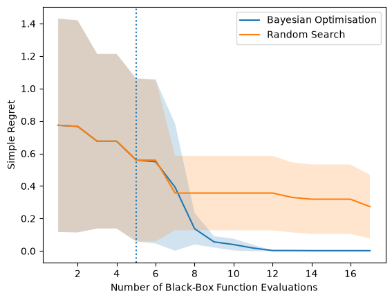
Finally, we'll process the experiment results to find the (simple) regret at each iteration of the experiments. The simple regret is defined as the difference between the maximum value of the black-box function observed so far and the true global maximum of the black box function. Mathematically, at time \(t\), with observations \(\mathcal{D}_t\), for function \(f\) with global maximum \(f^*\), the regret is defined as:

\[\text{regret}_t = f^* - \max_{\mathbf{x} \in \mathcal{D_t}}f(\mathbf{x})\]

We'll then take the mean and standard deviation of the simple regret values across the 5 experiments.

def obtain_regret_statistics(
    experiment_results: List[gpx.Dataset],
    global_maximum: float,
) -> Tuple[Float[Array, "N 1"], Float[Array, "N 1"]]:
    regret_results = []
    for exp_result in experiment_results:
        observations = exp_result.y
        cumulative_best_observations = jax.lax.associative_scan(
            jnp.maximum, observations
        )
        regret = global_maximum - cumulative_best_observations
        regret_results.append(regret)

    regret_results = jnp.array(regret_results)
    regret_mean = jnp.mean(regret_results, axis=0)
    regret_std = jnp.std(regret_results, axis=0)
    return regret_mean, regret_std


bo_regret_mean, bo_regret_std = obtain_regret_statistics(bo_experiment_results, 1.8377)
(
    random_regret_mean,
    random_regret_std,
) = obtain_regret_statistics(random_experiment_results, 1.8377)

Now, when we plot the mean and standard deviation of the regret at each iteration, we can see that BO outperforms random sampling!

fig, ax = plt.subplots()
fn_evaluations = jnp.arange(1, bo_iters + initial_sample_num + 1)
ax.plot(fn_evaluations, bo_regret_mean, label="Bayesian Optimisation")
ax.fill_between(
    fn_evaluations,
    bo_regret_mean[:, 0] - bo_regret_std[:, 0],
    bo_regret_mean[:, 0] + bo_regret_std[:, 0],
    alpha=0.2,
)
ax.plot(fn_evaluations, random_regret_mean, label="Random Search")
ax.fill_between(
    fn_evaluations,
    random_regret_mean[:, 0] - random_regret_std[:, 0],
    random_regret_mean[:, 0] + random_regret_std[:, 0],
    alpha=0.2,
)
ax.axvline(x=initial_sample_num, linestyle=":")
ax.set_xlabel("Number of Black-Box Function Evaluations")
ax.set_ylabel("Simple Regret")
ax.legend()
plt.show()

png

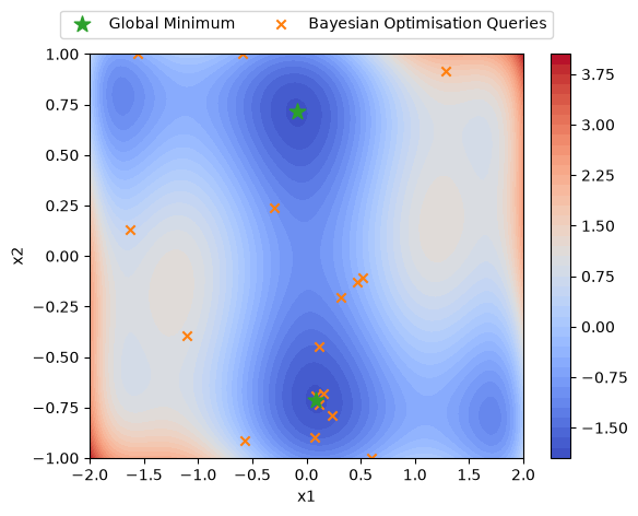
It can also be useful to plot the queried points over the course of a single BO run, in order to gain some insight into how the algorithm queries the search space. Below we do this for one of the BO experiments, and can see that the algorithm initially performs some exploration of the search space whilst it is uncertain about the black-box function, but it then hones in on the global minima of the function, as we would hope!

fig, ax = plt.subplots()
contour_plot = ax.contourf(
    x1, x2, y.reshape(x1.shape[0], x2.shape[0]), cmap=cm.coolwarm, levels=40
)
ax.scatter(
    x_star_one[0][0],
    x_star_one[0][1],
    marker="*",
    color=cols[2],
    s=120,
    label="Global Minimum",
    zorder=2,
)
ax.scatter(
    x_star_two[0][0], x_star_two[0][1], marker="*", color=cols[2], s=120, zorder=2
)
ax.scatter(
    bo_experiment_results[0].X[:, 0],
    bo_experiment_results[0].X[:, 1],
    marker="x",
    color=cols[1],
    label="Bayesian Optimisation Queries",
)
ax.set_xlabel("x1")
ax.set_ylabel("x2")
fig.colorbar(contour_plot)
ax.legend(loc="lower center", bbox_to_anchor=(0.5, 1.02), ncol=2)
plt.show()

png

System Configuration

%reload_ext watermark
%watermark -n -u -v -iv -w -a 'Thomas Christie'

Author: Thomas Christie

Last updated: Sat, 08 Aug 2026

Python implementation: CPython
Python version       : 3.13.15
IPython version      : 9.15.0

decijax   : 0.0.1
equinox   : 0.13.8
gpjax     : 0.15.0
jax       : 0.10.1
jaxtyping : 0.3.10
matplotlib: 3.11.0
paramax   : 0.0.5

Watermark: 2.6.0